From gigabytes of bird songs to a 60 kB model that runs on an ESP32
Introduction
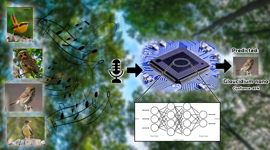
In recent years, artificial intelligence in microcontrollers (TinyML) has gone from being a laboratory curiosity to becoming a real tool for environmental monitoring, health, and industrial automation. This article shows how we transformed gigabytes of raw audio—the songs of six Patagonian species—into a fully INT8-quantized model that takes up just 60 kB of Flash and takes less than a second to classify a clip on an ESP32.
1. Why AI on the edge?
1. Latency & autonomy: Detecting a song or other key sound in < 1s allows for local action (activating a relay, turning on a LoRaWAN beacon).
2. Energy cost: Processing locally avoids transmitting complete spectrograms; we send only the tag and a score → fewer bytes, more battery life.
3. Remote coverage: An ESP32‑S3 + LoRa works where the cloud does not. Your proof of concept scales to hundreds of points
2. What are we working on?
• Taming an unbalanced dataset
The problem is the unbalanced ratio between recordings of the most abundant species and the rarest ones, where we have much more of the former and very little of the latter. If we train the model this way, it would learn to “play it safe”: it would mark almost everything as the dominant species and fail precisely when detecting rare songs. To level the playing field, we use controlled augmentation, generating synthetic examples—time-stretch, pitch-shift, and some pink noise—until each species has, for example, 500 clips. This way, the model receives the same number of examples per species, learns the characteristics of each song, and is not biased toward the most frequent birds.
• Using MFCC instead of a raw spectrogram
MFCCs (Mel Frequency Cepstral Coefficients) are a compact representation of a sound's spectrum that captures the acoustic characteristics as perceived by the human ear. MFCCs concentrate vocal energy into coefficients per frame, which reduces memory by a factor of 10 compared to a linear spectrogram. In addition, their 2-D format fits perfectly into lightweight 2-D CNN layers.
• In a minimalist 2-D CNN
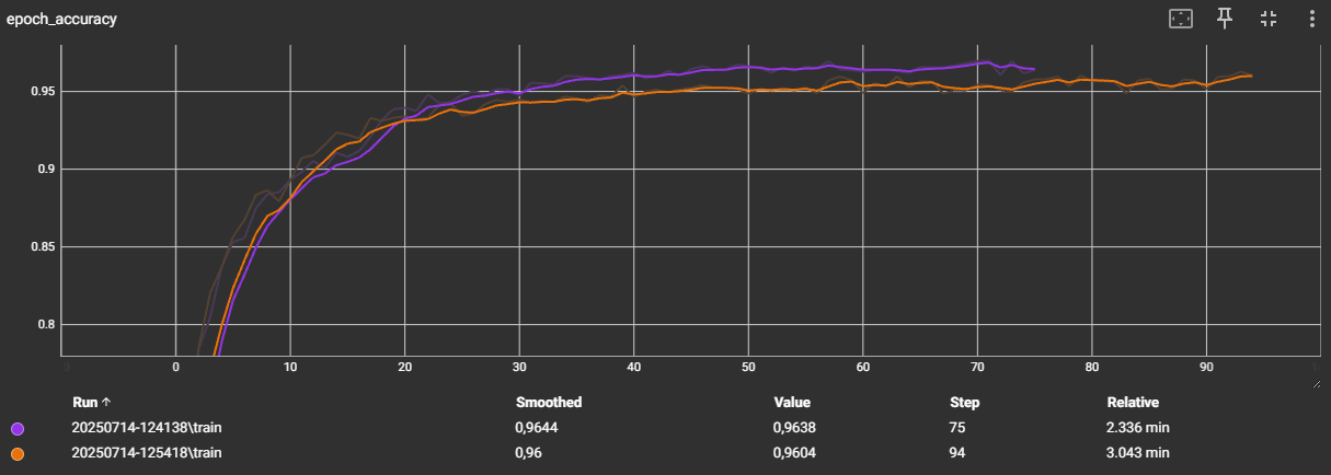
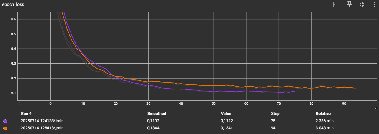
Convolutional layers allow the model to perceive when a sound occurs and what tone it has; with only 17,000 internal weights, we achieved more than 95% accuracy in species identification, keeping the model light enough (60 kB of Flash) to run smoothly on TFLite-Micro on a microcontroller.
• Measuring on the microcontroller before claiming victory
Simulating on the PC can be misleading: the cache, effective RAM, and DMA of the ESP32 alter the times. That's why we measure the inference on the microcontroller itself and monitor the TFLite-Micro tensor arena—the reserved memory block where all the model's intermediate tensors are stored—to adjust latency and confirm that the solution fits smoothly into the available memory.
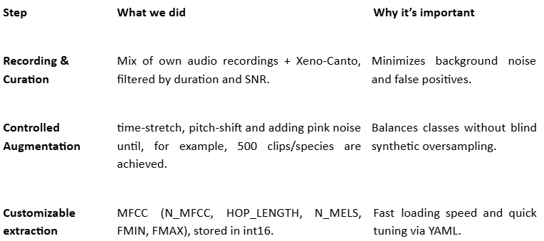
The pipeline allows you to easily change N_MFCC, HOP_LENGTH, N_MELS, frequency range, or even use linear spectrograms, and rebuilds the entire dataset.
4. Model comparison and selection guided by the pipeline
Our pipeline automates the entire experiment: it trains several architectures, generates metrics and graphs, and finally, with the results displayed, we can determine which models are worth porting to the microcontroller.
How does the flow work?
- Trains + validates each model with early stopping and saves the best checkpoint.
- Calculate complete metrics (AUC, F1, confusion matrix) and export them as PNG for quick inspection.
- Record resources: estimate the final size in Flash/RAM and inference time.
This way, we move from exploration on a PC to actual testing on a microcontroller.
5. Post-training quantization (full-INT8)
We opted for post-quantization with a representative set of, for example, 5000 spectrograms:
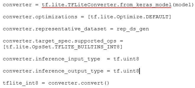
- -90% weight in Flash.
- Loss of only 0.4 pp in macro-AUC compared to float32.
- No modification of the original Keras code.
AUC = Area Under the Curve (0 = random, 1 = perfect). 0.95 ⇢ 95% average accuracy.
5. Deployment on ESP32-S3
Hardware
• ESP32-S3 @ 240 MHz
• I²S microphone @ 16 kHz mono
• SD card for logs and configurations
Zephyr integration
/* Pseudocode */
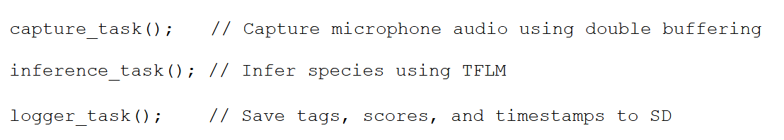
Measured results
- Total flash: 60 kB model + 4 kB TFLM code.
- RAM: 34 kB (for the model).
- Latency: 0.9 s per 3 s clip (continuous audio).
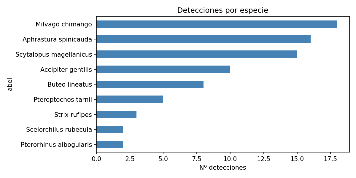
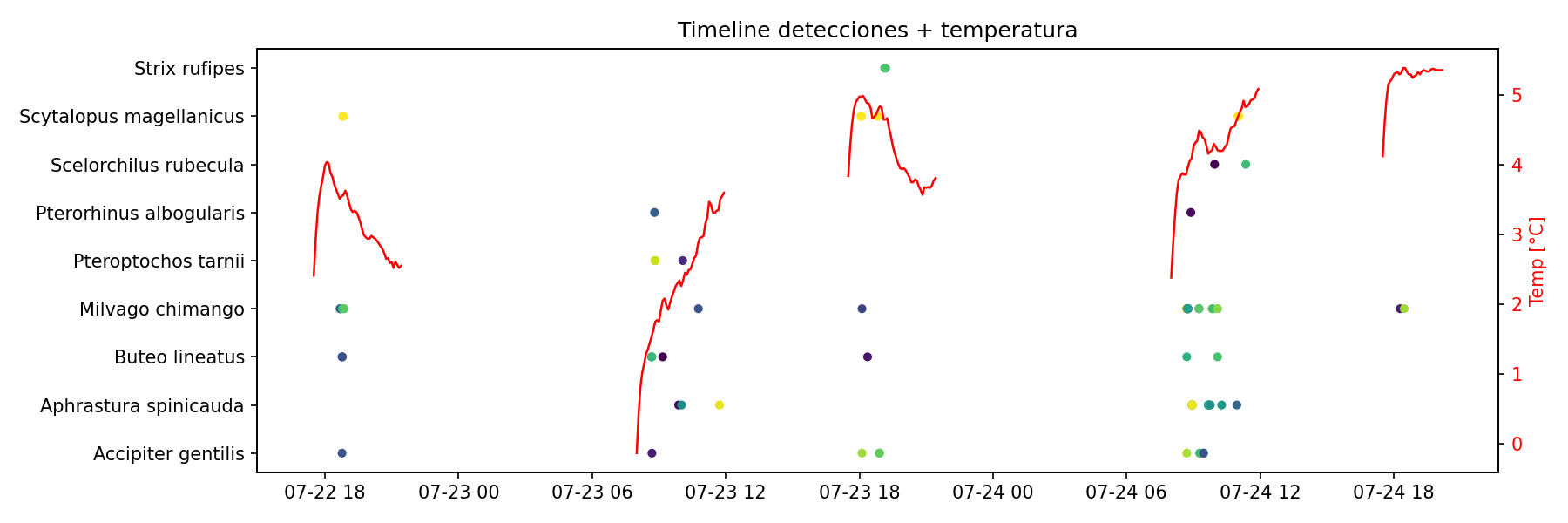
Some of the detected birds:
%20(1).jpg)
.jpg)
#TinyML #EdgeAI #ArtificialIntelligence #AI, #Engineering #Microcontrollers #TensorFlowLite #Conservation
Written by Alejandro Casanova
Embedded System Engineer at EmTech S.A
Any Comments or questions, please feel free to contact us: info@emtech.com.ar